10 Benefits of Custom Software for Your Business – Fewer Resources, Greater Efficiency
Dedicated software is an investment that increases company efficiency, minimizing IT resource consumption and supporting a sustainable development strategy.
 Author:
Today, we’d like to take you a little… deeper into the world of deep learning, specifically: artificial neural networks. Bear with us!
The internet is flooded with countless articles about the construction, operation, and training of neural networks. The authors typically aim to introduce readers to all the intricacies of these specific data processing structures, and there are indeed many of them. For someone approaching this topic for the first time, phrases like “chain rule” or “computing the gradient of the loss function” along with extensive calculations and formulas can be intimidating and discouraging, making you think, “this might not be for me…”. Often, people promise themselves to come back to the subject when they have more time, only to forget about it entirely (if they ever return at all). So, to avoid having extensive mathematical derivations that can discourage uninitiated readers, especially when it’s their first encounter with artificial neural networks, we’d like to propose an introduction of a more… gentle form.
Now that we’ve established the complexity of the topic we’re about to dive into, it’s time to lay out a plan that will help us navigate this challenging subject.
Starting with the end in mind, the first step is to determine the primary use cases for these networks and understand how an already trained model operates.
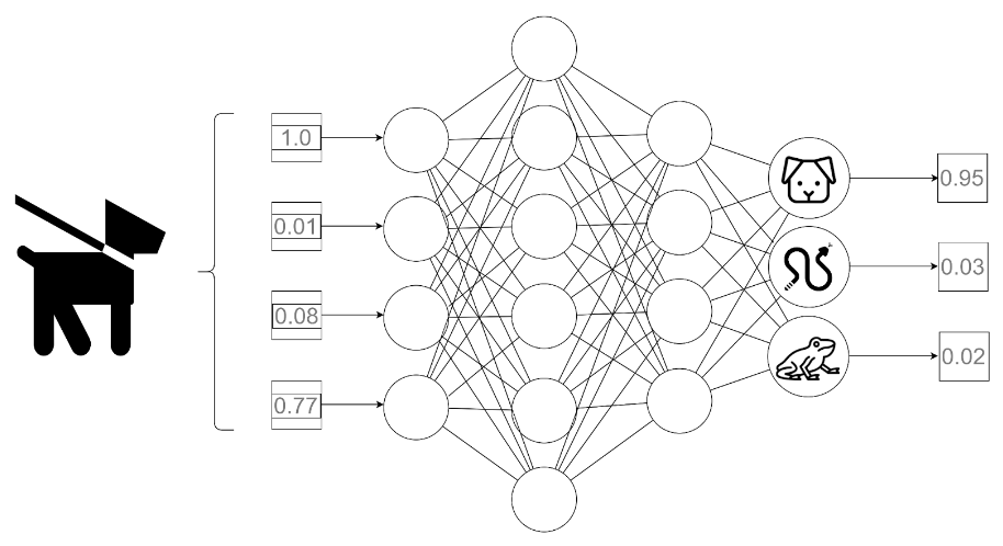
Although there are many variations of neural networks, we will focus on the most fundamental one, the Fully Connected Neural Network (FCNN), which is commonly used for classification. Classification involves assigning a data sample to a specific output category. This type of network takes an input vector of numbers and outputs the probabilities of the input belonging to each of the available classes.
For example, if we have input data describing the numerical features of an animal and the available classes are mammal, reptile, and amphibian, the network’s output would be the probability of the described organism belonging to each of these categories. Naturally, the final result would be the class for which the probability is the highest.
The process of assigning a specific class to a data sample by a trained model is called prediction.

Fig. 1: Schematic representation of the prediction process. A numerical feature vector of a dog is passed as input to the model. The output provides probabilities for the dog belonging to different classes.
We now know the use of FCNN, but we have yet to delve into how we obtain class probabilities from the input vector.
A neural network can be thought of as a massive, complex mathematical function that involves numerous linear operations (multiplication and addition) alternated with nonlinear operations.
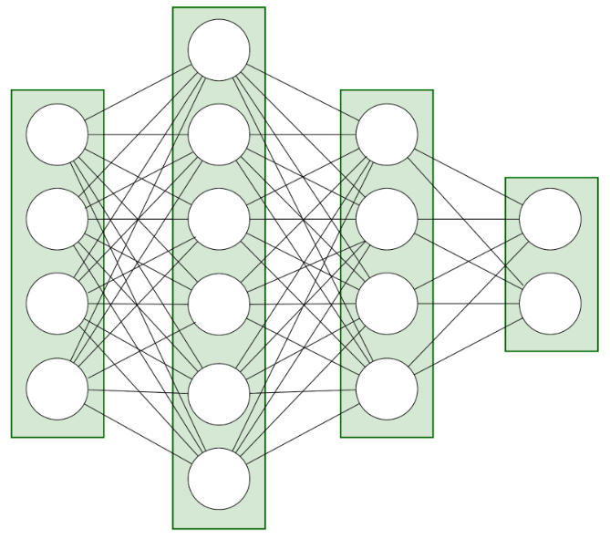
The network’s structure consists of layers with neurons, which are kind of computational nodes.

Fig. 2: Neural network layer structure – this example network consists of 4 layers: input, output, and two hidden layers.
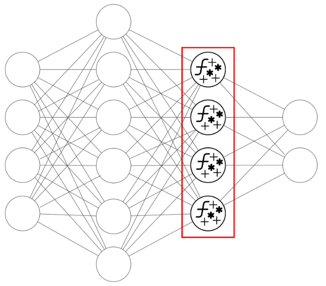
Each neuron defines a set of operations:
The output of a neuron is one of the elements passed to the next layer or to each neuron of the next layer. The entire process described above is repeated for each neuron in the following layer.

Fig. 3: Each neuron serves as a computational node, receiving and combining as many values as there are neurons in the previous layer (or, in the case of the first layer, as many as there are elements in the input vector). It then returns a single value, which is passed to each neuron of the next layer.
Even without a detailed analysis, it’s clear that the network operates by subjecting each input value to a series of operations, and each operation carrying its own weight. In an untrained network, these weights are initially assigned randomly, and thus, the results are also random. In a network trained for a specific task, the weights are adjusted to make the network provide highly confident responses on the final layer (i.e., the probability of one correct class being close to 1, while the others are close to 0).
Today, we’ve provided an overview of the prediction process in neural networks, and we now have a general understanding of how class probabilities are obtained from a data vector. In the next week, we’ll delve into the training of such networks. See you then!

10 Benefits of Custom Software for Your Business – Fewer Resources, Greater Efficiency
Dedicated software is an investment that increases company efficiency, minimizing IT resource consumption and supporting a sustainable development strategy.
Green IT

Responsible Software Development: How to Reduce Your Application’s Carbon Footprint?
Practical tips on how developers can actively reduce CO2 emissions by optimizing code, infrastructure, and application architecture.
Green ITInnovation

Green IT: How Technology Can Support Environmental Protection?
An introduction to the idea of Green IT – a strategy that combines technology with care for the planet.
Green ITInnovation